As Seasons Change So Does Your Data

Repeating, predictable patterns in data over a period of time, typically 12-months or more, are commonly characterized as seasonality. It’s certainly not the seasonal Fall or Autumn collection of the Vogue fashion trends which will never be repeated on the runway, but it’s the same predictable pattern every period. Since the oscillating highs and lows are tremendous, it is difficult to know if the good periods are actually that good or the bad periods are really that bad.

Seasonality can be present in virtually any type of data but it is most often associated with sales patterns. Forecasting and analyzing such seasonal sales data can only be an exercise in futility without first some type of de-seasonalization process to normalize the data. The way to move forward is to identify a seasonality sales trend, de-seasonaliz the sales data, analyze and forecast the data and then re-seasonalize the trend to arrive at your final financial forecast.

Simplest Form of De-Seasonalization

When analyzing data, and not forecasting, the simplest and easiest thing you can do is measure against the same period in the last cycle. For example, January current year against January last year. This has obvious flaws, in the current or prior period there could have been a recession or a boom year and therefore by biased toward one way or the other giving your analysis less weight.

In addition, progression from prior period is also a metric that many senior executives like to see. The ability for them to sell the board or their investors that the organization is doing better than the comparison period is always a feather in their cap, regardless of the true reason. As a Financial Planning and Analysis (FP&A) or internal Corporate Finance professional your analytic abilities to discern the difference between luck and skill is subjective and should be taken into account depending on what Prince you may be serving.

Seasonality in Action

We are going to use an experiment here to de-construct seasonality. I utilized the sales data for a 5-year period and have explained via screenshots the steps to be followed.

Points to be noted: Please note that the span of data should have an equal number of annual data points to avoid skewing the data. For e.g. – let there be an equal number of January data points or an equal number of December data points. We are taking data from Jan 2009 to Dec 2013.

Create a pivot table as shown below with row labels of months and sales data as column information.

Do this by selecting your data and then moving your cursor up into the Excel ribbon and selecting Insert – Pivot Table, shown below

If Excel does not automatically place your data into groups, select the “Row Labels” column, right click on the Pivot table and go to ‘Group’. Choose ‘Months’ in the menu as shown below

This will produce a table with the sum total of sales by month that looks as like this:

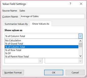
Now we need the Sum of Sales column to be represented as a percentage of the Grand Total column. To do this, we click on any number in the pivot table to bring up the Filed List window, select Sum of Sales and choose Value Field Settings.

Within the Value Field Settings choose Average

Then click on the Show Values As tab and select % of column Total, then press OK

This will produce the sensualized index table as shown below, with total monthly average sales of 100%.

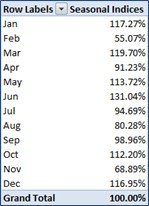
The seasonalized index will now be the fulcrum by which you will de-seasonalize historical data, forecast future sales and then re-seasonalize the data to base future financial forecasts. This index should be periodically revisited to capture changes that occur from one cycle to the next. For example, it makes sense to update only once a full cycle’s data can be included but not mid-cycle as that may skew the forecast data and provide confusion to users. 5 Historical sales figures should be divided by the seasonal index for that month which gives you historical de-seasonalized sales.

Pulling data from a pivot table can be kind of tricky so to help do this we use a smart trick of the INDEX function which picks up the data for the correct month by using the reference of the MONTH formula from the correct row in the pivot table. Just be careful to lock the range of the pivot data.

Forecast The De-seasonalized Sales Data: Excel 2016 has added some great new forecasting features and you can forecast using n moving average or many other techniques, but for this example we are focusing on seasonality, so we are going to use a simple linear regression formula. In Excel 2016, the Formula is FORECAST.LINEAR and in earlier versions of Excel the formula is just FORECAST.

Forecast the next 12-months of sales and then de-seasonalize the sales data by multiplying the forecasted sales data by the seasonal index to get your final monthly financial forecast number.

There you have it!

You have taken time series sales data, de-seasonalized it, forecasted it and re-seasonalized it into a financial forecast but does it make sense? Looking at the chart below, it does not look way off, but it certainly looks a lot less volatile than previous periods, which brings up a lot of questions.

Before presenting any financial forecast sufficient due diligence as to the supporting assumptions and the basis of ones conclusions should be performed. Being wrong is part of financial forecasting but not having a basis for why you are wrong is never a good idea in general.

You can find the complete Excel spreadsheet with the supporting formulas and charts by clicking here.

What other templates and processes would you find useful to help you in your job? Let me know in the comments below.